Custom metrics
Every machine learning model is unique and no monitoring solution is one size fits all. MPM tracks feature distributions, data drift and accuracy metrics out of the box, but sometimes you need more. This is where MPM Custom Metrics come in.
Custom metrics are written in a SQL-like language and created from the MPM settings tab.
Writing a custom metric
Custom metrics are defined in the MPM settings tab under Custom Metrics.
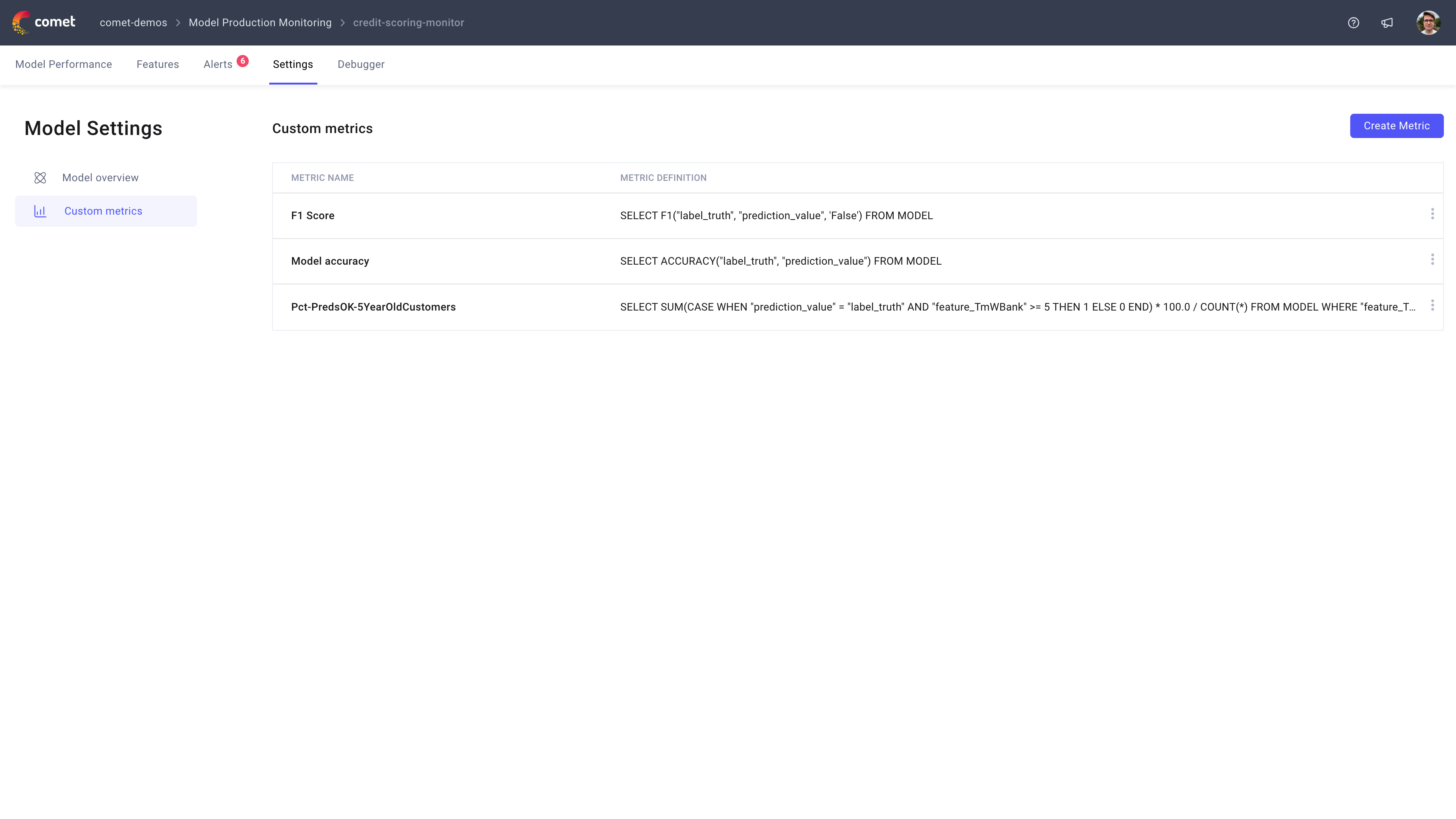
You give the metric a name and a formula. A custom metric follows this format:
SELECT
    <METRIC FORMULA>
FROM
    MODEL
WHERE
    <OPTIONAL FILTER>
MODEL is a keyword standing in for your model's event table — you never name a table.
Note
The metric formula needs to be an aggregation over your predictions or labels that returns a single value. That value is what gets plotted for each hour or day.
While writing the definition you can preview the metric on the right hand side of the screen.
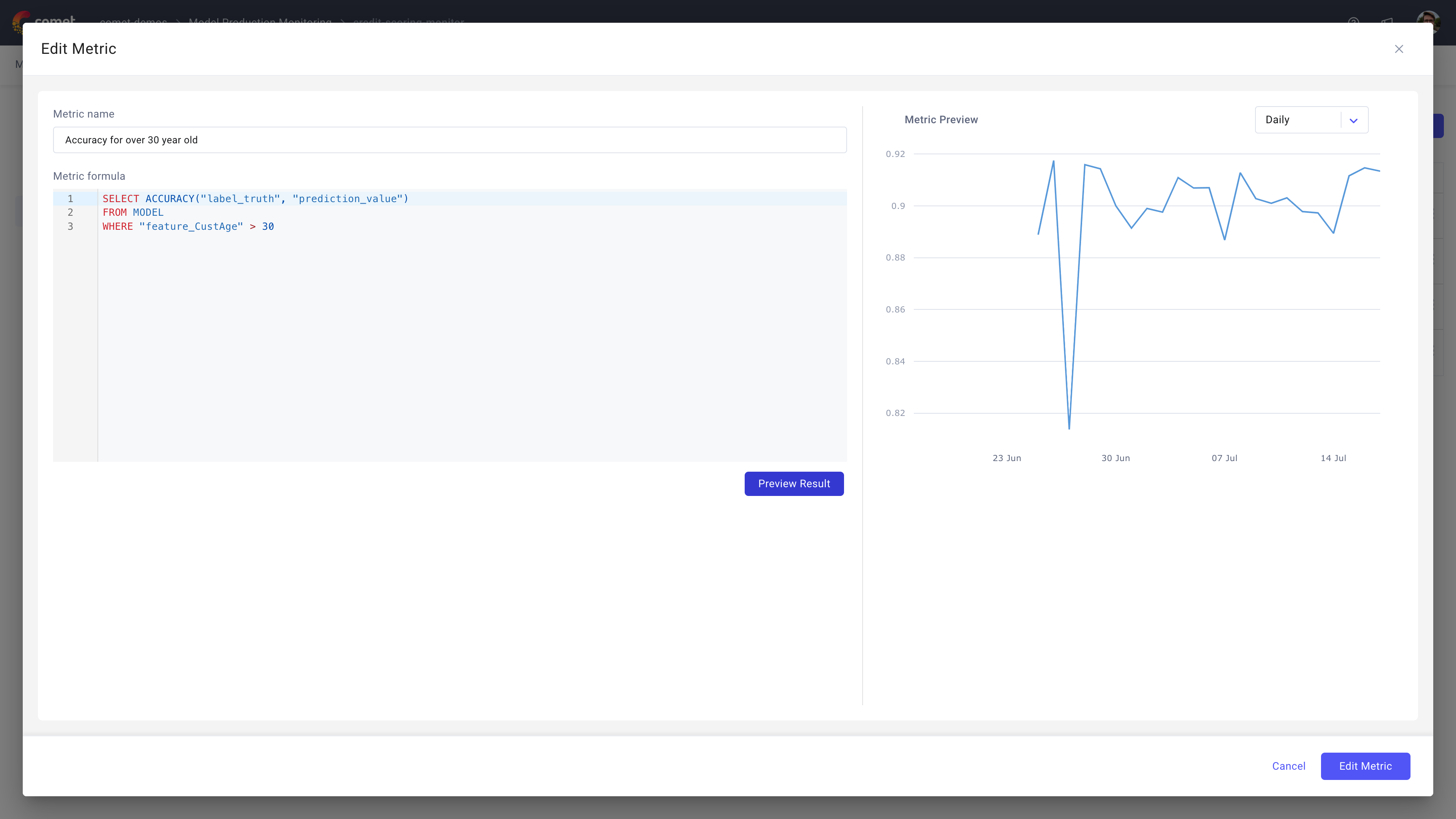
Once saved, the metric appears on the Model Performance page. MPM converts your formula into a database query based on the options you have selected — hourly versus daily, a specific model version, any dashboard filters.
Note
You can create an alert on any custom metric you have created.
Referring to columns
Column names always carry their prefix and are wrapped in double quotes:
| Prefix | Meaning | Example |
|---|---|---|
feature_ | An input to the model | "feature_CustAge" |
prediction_ | An output of the model | "prediction_score" |
label_ | Ground truth | "label_response" |
Naming your metrics
Use AS to name a metric. The name appears in the chart legend, and is what you select when creating an alert on a query that contains several metrics:
SELECT COUNT(*) AS total,
       AVG("feature_CustAge") AS avgAge
FROM MODEL
Note
A query may contain several metrics separated by commas. Without a name, a metric is labelled with its formula text, which is valid but harder to work with.
An unquoted name is upper-cased, the usual SQL rule. AS avgAge becomes AVGAGE in the legend and in the alert's metric list. To keep the capitalisation you wrote, quote it:
| Written | Appears as |
|---|---|
AS avgAge | AVGAGE |
AS "avgAge" | avgAge |
Either works. It is worth settling on one before you create alerts, since the alert names the metric as the chart does, and a name that changes shape between the two is needlessly confusing to read.
Example custom metrics
A metric over a subset of predictions
Use the WHERE clause to compute a metric over a subset of the predictions:
SELECT COUNT(*)
FROM MODEL
WHERE "feature_CustAge" > 30
Note
To compute the percentage of predictions with a certain value, use a CASE statement in the SELECT clause instead:
SELECT SUM(
    CASE WHEN "feature_TmWBank" >= 5
         THEN 1
         ELSE 0
         END) * 100.0 /
  COUNT(*) FROM MODEL
Filtering one metric without filtering the others
FILTER (WHERE ...) narrows a single metric, leaving the others in the query untouched:
SELECT COUNT(*) AS total,
       COUNT(*) FILTER (WHERE "feature_country" = 'UK') AS ukOnly
FROM MODEL
A dashboard filter applied to the chart narrows this further rather than replacing it — see Combining with filters you wrote yourself.
A running total
OVER (ORDER BY timeBucket) accumulates a metric across time buckets:
SELECT SUM("feature_amount") OVER (ORDER BY timeBucket) AS cumulativeAmount
FROM MODEL
See Window functions for rolling windows and the rules that apply.
Model performance functions
MPM provides functions for common machine learning metrics.
Note
The label comes first, then the prediction. For the per-class functions, the third argument is the class value the metric is computed for.
Classification, computed for one class
| Function | Meaning |
|---|---|
PRECISION(label, prediction, class) | Precision for that class |
RECALL(label, prediction, class) | Recall for that class |
F1(label, prediction, class) | F1 score for that class |
TPR(label, prediction, class) | True positive rate |
FPR(label, prediction, class) | False positive rate |
TNR(label, prediction, class) | True negative rate |
FNR(label, prediction, class) | False negative rate |
SELECT F1("label_response", "prediction_class", 'fraud') AS f1Fraud
FROM MODEL
Precision for which class? is a question every classification metric has to answer, which is why these take a class value.
Overall accuracy and regression error
| Function | Meaning |
|---|---|
ACCURACY(label, prediction) | Proportion of predictions matching the label |
MAE(label, prediction) | Mean absolute error |
MAPE(label, prediction) | Mean absolute percentage error |
RMSE(label, prediction) | Root mean squared error |
MAX_ERROR(label, prediction) | Largest single error |
SELECT ACCURACY("label_response", "prediction_class") * 100 AS accuracyPct
FROM MODEL
Scoring predicted probabilities
| Function | Meaning |
|---|---|
LOG_LOSS(label, prediction_probability, class) | Logarithmic loss for that class |
LOG_LOSS is the one function whose second argument is a probability rather than a predicted class — the number your model gave for the class named in the third argument:
SELECT LOG_LOSS("label_response", "prediction_probability", 'fraud') AS logLoss
FROM MODEL
It rewards being confident and right, and penalises being confident and wrong, far more sharply than accuracy does. A model that says 0.99 and is wrong scores much worse than one that says 0.6 and is wrong.
Aggregations and maths
Model performance functions combine with ordinary aggregations and arithmetic.
Aggregations
COUNT, SUM, MIN, MAX, AVG, APPROX_COUNT_DISTINCT, STDDEV_POP, STDDEV_SAMP, VAR_POP, VAR_SAMP, and APPROX_QUANTILE_DS(column, quantile).
SELECT APPROX_QUANTILE_DS("prediction_score", 0.95) AS p95Score
FROM MODEL
Maths functions
ABS, CEIL, FLOOR, EXP, LN, LOG10, SQRT, POW(x, n), GREATEST(...), LEAST(...), and the operators + - * / ^.
Conditionals
CASE WHEN ... THEN ... ELSE ... END, as in the percentage example above.
These compose, so a performance function can sit inside arithmetic or an aggregation:
SELECT RECALL("label_response", "prediction_class", 'fraud') / SQRT(COUNT(*)) AS scaledRecall
FROM MODEL
Dividing whole numbers
Dividing one whole number by another gives a whole number, and the remainder is discarded rather than rounded. COUNT returns whole numbers, so a ratio of two counts is the first place this bites:
-- 2191 out of 4000 predictions, charted as 0
SELECT COUNT(*) FILTER (WHERE "feature_amount" > 1000) / COUNT(*) * 100 AS pctLarge
FROM MODEL
2191 / 4000 is 0 before the multiplication ever happens, so the metric charts a flat zero. It is not rejected, because nothing about it is invalid — it is arithmetic doing exactly what it was asked.
Introduce the decimal first, and the division keeps its fraction:
-- 54.775
SELECT COUNT(*) FILTER (WHERE "feature_amount" > 1000) * 100.0 / COUNT(*) AS pctLarge
FROM MODEL
Note
100.0 rather than 100, and placed before the division rather than after it. This is why the percentage example earlier in this page multiplies by 100.0. A metric stuck at 0, or one whose line only ever takes whole-number steps, is almost always this.
AVG is safe whatever it averages, because it returns a decimal on its own. SUM is not: it returns whatever kind of number the column holds, so SUM of a decimal column divides cleanly while SUM of a whole-number column has the same problem as COUNT.
-- "label_response" holds 0 and 1, so this proportion charts as 0
SELECT SUM("label_response") / COUNT(*) AS positiveRate FROM MODEL

-- 0.227
SELECT SUM("label_response") * 1.0 / COUNT(*) AS positiveRate FROM MODEL
Dividing by zero
A bucket whose denominator comes out as zero fails the whole chart rather than that one point. Denominators that are normally safe can still reach zero in a quiet hour, or under a dashboard filter that matches very little.
Guard the denominator with NULLIF, which turns a zero denominator into no value rather than an error:
SELECT SUM("feature_amount") / NULLIF(COUNT(*) FILTER (WHERE "prediction_decision" = 'approve'), 0)
       AS avgApprovedAmount
FROM MODEL
CASE WHEN ... THEN 0 ELSE ... END works equally well. Either way the guarded bucket is charted as 0, so read a zero here as "nothing to divide by", not as a measurement — the two are worth telling apart when the metric is a rate that could legitimately be zero.
What happens to your formula
MPM wraps your formula in a larger query before running it, and the shape of that wrapper explains most of the rules above. For:
SELECT AVG("feature_amount") AS avgAmt FROM MODEL
with a dashboard filter for UK-only predictions, MPM generates approximately:
SELECT <time bucket> AS timeBucket,
       AVG("feature_amount") FILTER (WHERE true = true)               AS "…all…AVGAMT",
       AVG("feature_amount") FILTER (WHERE "feature_country" = 'UK')  AS "…uk-only…AVGAMT"
FROM   <your model's events>
WHERE  <the selected time range>
GROUP BY timeBucket
Your metric is computed once per filter, and the whole query is grouped into time buckets. That is why a formula has to reduce to a single value, and why extra dashboard filters cost so little — they become columns in one query rather than separate queries.
Where the dashboard filter lands
The example above has a single aggregation, which hides a detail worth knowing: the filter is applied to each aggregation in your formula, not wrapped around the formula as a whole.
For a ratio, both halves are filtered:
SELECT SUM("feature_amount") / COUNT(*) AS avgTicket FROM MODEL
SUM("feature_amount") FILTER (WHERE "feature_country" = 'UK')
  / COUNT(*) FILTER (WHERE "feature_country" = 'UK')
This is the only reading that means anything. Filtering one side and not the other would divide a UK-only total by a count of every prediction — a number that is not the average of anything.
The same holds for arithmetic around an aggregation. In AVG("feature_amount") * 100 the filter attaches to the AVG, not to the * 100, because multiplying by a hundred is not something a row can be filtered out of.
Note
A metric carrying several aggregations is filtered consistently — all of them, or none. There is no way to write a formula where the dashboard filter reaches some aggregations but not others, and that is deliberate.
Combining with filters you wrote yourself
A dashboard filter never replaces a condition in your formula. It narrows it. Whichever way you have restricted the rows, the two conditions are combined with AND and you see the overlap.
That applies to both places you can write a condition:
| In your formula | With a dashboard filter for country = 'UK' | Rows counted |
|---|---|---|
COUNT(*) | — | UK |
COUNT(*) FILTER (WHERE "feature_amount" > 1000) | — | UK and over 1000 |
COUNT(*) FROM MODEL WHERE "feature_amount" > 1000 | — | UK and over 1000 |
So a metric written as "approved predictions" charted under a dashboard filter for the UK shows approved UK predictions, not all approvals and not all UK predictions.
Note
This is worth checking when a number looks smaller than you expected. A metric that already filters, viewed under a dashboard filter that also narrows, can leave very few rows — and a bucket with no matching rows has no point on the chart rather than a zero.
In a query with several metrics, each is filtered independently, so a metric carrying its own FILTER and one without it can sit side by side and both behave correctly:
SELECT COUNT(*) AS total,
       COUNT(*) FILTER (WHERE "prediction_decision" = 'approve') AS approved
FROM MODEL
Under a dashboard filter, total counts the filtered rows and approved counts the filtered rows that were also approved.
Validation
Metrics are checked in three places:
- As you type, the editor underlines anything malformed, and explains the rules it can check — such as an argument that should be a label column but is not.
- When you save, the formula is parsed and rejected if it cannot be run. This matters because a metric that only failed when charted would also fail inside an alert, where nobody is watching.
- When charted, as a final check.